�ҡ@�@�{�G�t��k ���ɱЮv�G�����C �t�@�@�šG��u�դT �m�@�@�W�G�c�|�s �ǡ@�@���G8834809
Voronoi Diagrams( Apply to Mobile Phone Position
Located problem)
²���G
���ʹq�ܳq�T�������A�b�Y�ǯS�w���ݨD���]�Ѧp�G�D�ƿ�סB�Ҧb�a������T�d�ߪA�ȡB�K���^�A�ڭ̥����D�o��ʹq�ܩҳB��m�B�϶������D�C
���D�P��z�ѻ��G
���������D�̥D�n���O�n��D�o��ʹq�ܩ��T���ҳB�ϰ�A�B��d���Y�o�U�p�U�n�C�ڦ��A�ڭ̴��X�U�z���ѨM��סA��D���Voronoi Diagrams�BDelaunay Triangulation�P��������z�װ�¦�C�H�U�}�l������������¦�w�q�P�t��k�G
�b��ʹq�ܳq�T�������A��ʹq�ܺ��C���a�x�Ҳ[�\���A�Ƚd���A����b���@�����ҨϥΪ���a�x�A�O�b��ҷj�M�쪺��a�x�T���j�z�C�����]�@�묰�|��E�հ�a�x�^����T���̦n����a�x�ӵ��U�ϥΪA�ȡC
�]���A�w��H�W�S�ʡA�ڭ̱N�����D�ഫ���Voronoi Diagrams�����D�A
����Voronoi Diagrams���w�q�A�H�U�`���������C�б½ҵ{���q�Ĥ����G
l The Voronoi diagram problem
e.g.
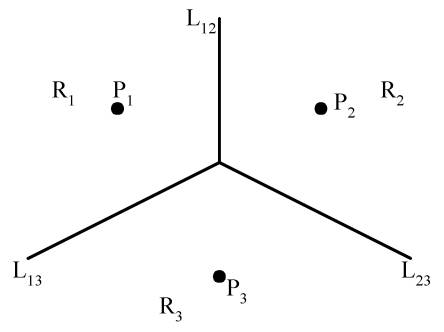
The Voronoi Diagram for Three Points
Each Lij is perpendicular bisector of the line ![]() .
.
Def: Given two points Pi, Pj Î S, let H(Pi, Pj) denote the half plane containing Pi. The Voronoi polygon associated with Pi is defined as
V(i)
= ![]() H(Pi,
Pj)
H(Pi,
Pj)
e.g.
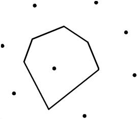
Given a set of n points, the Voronoi diagram consists of all the Voronoi polygons of these points.
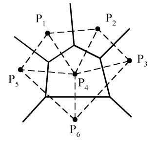
e.g. A Voronoi diagram of 6 points:

The vertices of the Voronoi diagram are called Voronoi points and its segments are called Voronoi edges.
e.g. A Delaunay triangulation:
�b���A�ڭ̱N���ѪA�Ȫ���a�x����Voronoi Diagrams���D�����U�I�A���]�C�Ӱ�a�x���o�g�\�v���ۦP�A�ӫت���q�i�T�����z�Z�i�������p�C����ʹq�ܶZ���Y�@��a�x����ɡ]�i�J�����դO�d��^�A�Ӱ�a�x���T���̱j�A�]���|�V�Ӱ�a�x���U�A�åѸӰ�a�x���ѪA�ȡA�ҥH�ڭ̭n�D�X�U�I���դO�d����G��Voronoi Diagrams�A�Y�i�o����ʹq�ܩҳB���ϰ�d��]�Ĥ@���^�C
![]()

�b��Voronoi Diagrams�����D�W�A�ڭ̥��D�X�U�I�ҹ�����Delaunay Triangulations�A����A�i�@�B�ϥιL�{���w�o���������u�B�~�ߡBvisible neighbors��������T�D�o�۹�����Voronoi edges�C�bDelaunay Triangulations���غc�W�ڭ̨ϥΪ��OBowyer-Watson Algorithm�C
���U�ӧڭ̰w��t��k���������i�@�B������
�t��k�G
Step 1
Define a bounding box that contains all
the points. This step is needed to initialise the algorithm by defining an
initial triangulation and associated topology.
One of the possibilities is to specify
four points together with the associated vertex and neighbours structure. The
Figure below shows a typical start-up layout for the two-dimensional case.
Another possibility is to define an initial simplex (a triangle in 2D) which contains all the points.
figure. a Start-up layout in two dimensions (4 points, 2 triangles)
Step 2
Introduce a new point anywhere within the
bounding box which, by construction, contains all the points.
Step 3
Find the first triangle that fails the
Delaunay test.
Step 4
Determine all triangles that make up the
Delaunay cavity ..
The remaining steps in the algorithm are
needed to update the data structure. Broken elements are deleted and new ones,
obtained by connecting the new point to all edges of the cavity, are created.
Finally it is necessary to determine the contiguities that exist between the
new elements and also between the new elements and the ones that are on the
boundary of the Delaunay cavity to update all topological relationships.
Step 5
Remove all triangles in the Delaunay
cavity.
Step 6
Connect the edges of the Delaunay cavity
with the new point to generate a new set of triangles.
Step 7
Update the neighboring information for the
new triangles and the elements at the boundary of the cavity.
Step 8
Goto Step 2
We now have a triangulation of the set of
points whose boundary is defined by the extent of the bounding box built at the
beginning of the procedure.
Step 9
If we remove from the list of triangles
all elements that share a vertex with the initial bounding box, we obtain a
Delaunay triangulation of the convex hull of the given set of points. We can
also extract the boundary of the triangulation to obtain a set of edges
defining the convex hull of the point set.
Definition 1:
Let T be a Delaunay triangulation and let��s consider a new point P inside T. Let B Ì T be the set of triangles which are broken by P because they fail the In-Circle criterion (section 2.4.2) . Clearly this set contains at least one member, the triangle that contains P (fig 2.10a-b). Once a first broken element is found, by following the explicit topological relationships of each triangle with its neighbours it is easy to find the whole set of elements that fail the In-Circle criterion. The region created by removing B from T is called a Delaunay cavity.
Definition 2:
The point A of a
triangle set is visible from another point B if it is possible to join A
to B without intersecting any other edge. For the Bowyer-Watson��s algorithm to
be valid, it is necessary that all points of all edges forming a Delaunay
cavity be visible from point P. The situation depicted below, for example,
where edge CD is not visible from P leads to an invalid triangulation in which
two or more edges intersect . It is also necessary that the new triangulation,
formed by connecting P to the boundary points of the cavity, also be Delaunay.
Baker (1987) contains
complete proofs for definitions 1 and 2 and why the procedure described
generates a valid Delaunay triangulation.
Definition 3:
Given a triangle
(ABC), the circumcircle of the triangle, the centre of the circumcircle V, and
a point P, the comparison of the distance between a point P and the
circumcentre V with the radius (r) of the circumcircle will be referred to as
the Delaunay test for the triangle (ABC) and point P. If a point is
found to lie inside the circumcircle then we can say that the point has failed
the Delaunay test for that particular triangle.
�{���]�p�G
The key issues of this algorithm about determining Delaunay cavity and Delaunay test function are implementing in isCross() and SetDelaunay() subfunctions.
There are some special exceptions need to take care during the implementation:
�P two points are coincident
The first degeneracy is easily avoided by
requiring that each new point be some small distance from its nearest
neighbours. The n-tree data structure provides a natural way of guaranteeing
this, in fact points are sifted into the data structure and those that are
"close enough" to each other (depending on the machine precision)
will end up in the same space partition. At this point a co-ordinates check
against all the points already in the tree node is done to guarantee
uniqueness. In this latest comparison operation an allowance is made to
compensate for lack of machine precision through the use of a precision
parameter e (epsilon),
so that co-ordinate whose absolute distance is less than e are considered equal.
�P three points of a potential triangle lie on a straight line
This degeneracy is equivalent to there not
existing a circumcentre of the three forming points of a potential triangle.
This case can be easily detected as the routine to compute the co-ordinates of
the circumcentre will fail. The point that causes the degeneracy is at first
temporarily excluded from the construction and another insertion attempt is
made at a later stage, if the problem still exists the point is then definitely
rejected. This is in practice a very rare case especially in two dimensions.
�P four or more points are cyclic
This third degeneracy is of a more subtle
nature than the preceding two. In this case two Voronoi vertices are coincident
and generate a case where more than three Dirichlet polygons meet (fig 2.15).
In such a situation the resulting triangulation is not unique due to a symmetry
in the data points but this in itself is not a problem as the two possible
triangulations are both correct and acceptable. Which one is then built will
depend on the order of insertion of the points.
���絲�G�G
Time Complexity Analysis:
To define the complexity
of the algorithm used in this implementation we need to highlight which
components are dependent on the number of points and therefore play an
important part in the complexity equation. With the exception of Step 3, all
the operations required are of a local nature and can be carried out in a time
independent of the total number of points within the current structure. When a
new point is inserted, we first have to search for the first element that fails
the Delaunay test. The other elements in the Delaunay cavity can be found using
a recursive search of the neighbors of the first element found if we maintain a
topological relationship among the elements so that each triangle also stores
the reference to all its neighbors.
We can define the time
T needed to generate a triangulation for N points as :
where Tk is the time to find the first element to be deleted and Sk the time to find all the other elements in the cavity. Sk will be proportional to the number of elements in the cavity, this can be considered independent from k if the points are inserted randomly into the triangulation (Baker, 1987). This means that we can consider Sk as being O(1). We can see now that the complexity of the algorithm is dominated by the search time Tk. In the worst case Tk will be O(k) leading to a total complexity of the triangulation of O(N2). To improve the time complexity of the algorithm it is then necessary to implement a data structure that allows an efficient search of the first element to be deleted independently from the way the points are sorted. If the search time Tk can be reduced to logN we could obtain a time complexity for this algorithm close to the theoretical optimum of O(NlogN).
���פ߱o�G
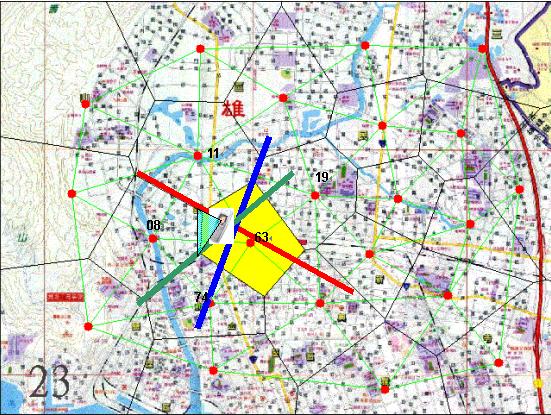
��project���Ĥ@���O�ھڦ�ʹq�ܻP��a�x�����S�ʥi�PVoronoi Diagrams�����D�۹����ӸѨM��Position Locating�����D�A�����b��ʹq�ܨ�ҷj�M�쪺��a�x�T���j�z�C�����]�@�묰�|��E�հ�a�x�^���t�F���״I����T�i�ΨӶi�@�B���Y�p��Ҧb���a�z�d���T�A�]�N�O���A�ڭ̥i�H�ޥΥثe�Ҧb����a�x�]63�^������Delaunay Triangulations����a�x��T�]�p�G11�B08�B19�B74�B�K���^�P��ʹq�ܤW����a�x�T���j�z�C���]�p�G63 > 08 > 11 > 74 > 19�^�C�ڦ��A�H�U�Ϭ��ҡA�ڭ̴N�i�H�N��ҳB���a��d��j�T�Y���L���h��Ϊ��d��A�o�O�ڭ̲ĤG���n�����������]To be continued�K�^�C
i.e. : ���k�Y���ΦbPHS�C�\�v��ʳq�T���ҤU�A�Y�p���d��N����ۡA�]���ثe�U�a�t�өҥͲ���PHS��a�x�ү�[�\���d��ɩ�@�줭�ʤ��ؤ����C
�����G
��l�{���X�]Java�^�GMPLocating.java
�����a�ϡGKSMap.gif
Java applet: MPLocating.class
On-line Applet�G
|
|